Introduction to Data Science - Unit : 2 - Topic 7 : CASE STUDIES ON DS PROJECTS FOR PREDICTING MALICIOUS URLS FOR BUILDING RECOMMENDER SYSTEMS

 

CASE STUDIES ON DS PROJECTS FOR PREDICTING MALICIOUS URLS

FOR BUILDING RECOMMENDER SYSTEMS

 

Case study 1: Predicting malicious URLs

The internet is probably one of the greatest inventions of modern times. It has boosted humanity’s development, but not everyone uses this great invention with honorable intentions. Many companies (Google, for one) try to protect us from fraud by detecting malicious websites for us. Doing so is no easy task, because the internet has billions of web pages to scan. In this case study we’ll show how to work with a data set that no longer fits in memory.

What we’ll use

Data—The data in this case study was made available as part of a research project. The project contains data from 120 days, and each observation has approximately The 3,200,000 features. The target variable contains 1 if it’s a malicious website and -1 otherwise. For more information, please see “Beyond Blacklists:Learning to Detect Malicious Web Sites from Suspicious URLs.”2

The Scikit-learn library—You should have this library installed in your Python environment at this point, because we used it in the previous chapter.

Step 1: Defining the research goal

The goal of our project is to detect whether certain URLs can be trusted or not. Because the data is so large we aim to do this in a memory-friendly way. In the next step we’ll first look at what happens if we don’t concern ourselves with memory (RAM) issues.

Step 2: Acquiring the URL data

Start by downloading the data from http://sysnet.ucsd.edu/projects/url/#datasets and place it in a folder. Choose the data in SVMLight format. SVMLight is a text-base format with one observation per row. To save space, it leaves out the zeros.

            TOOLS AND TECHNIQUES

We ran into a memory error while loading a single file—still 119 to go. Luckily, we have a few tricks up our sleeve. Let’s try these techniques over the course of the case study:

Ø  Use a sparse representation of data.

Ø  Feed the algorithm compressed data instead of raw data.

Ø  Use an online algorithm to make predictions.

Step 4: Data exploration

To see if we can even apply our first trick (sparse representation), we need to find out whether the data does indeed contain lots of zeros. We can check this with the following piece of code:

print "number of non-zero entries %2.6f" % float((X.nnz)/(float(X.shape[0]) * float(X.shape[1])))

This outputs the following:

number of non-zero entries 0.000033

Data that contains little information compared to zeros is called sparse data. This can be saved more compactly if you store the data as [(0,0,1),(4,4,1)] instead of [[1,0,0,0,0],[0,0,0,0,0],[0,0,0,0,0],[0,0,0,0,0],[0,0,0,0,1]]

Part of the code needs some extra explanation. In this code we loop through the svm files inside the tar archive. We unpack the files one by one to reduce the memory needed. As these files are in the SVM format, we use a helper, functionload_svmlight _file() to load a specific file. Then we can see how many observations and variables the file has by checking the shape of the resulting data set.

Step 5: Model building

Now that we’re aware of the dimensions of our data, we can apply the same two tricks (sparse representation of compressed file) and add the third (using an online algorithm), in the following listing. Let’s find those harmful websites!

Here, we trained the algorithm iteratively by presenting the observations in one file with the partial_fit() function. Looping through only the first 5 files here gives the output shown in table 4.1. The table shows classification diagnostic measures: precision, recall, F1-score, and support.

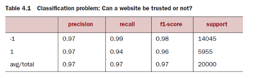
Only 3% (1 - 0.97) of the malicious sites aren’t detected (precision), and 6% (1 - 0.94) of the sites detected are falsely accused (recall). This is a decent result, so we can conclude that the methodology works.

Case study 2: Building a recommender system inside a database

In reality most of the data you work with is stored in a relational database, but most databases aren’t suitable for data mining. But as shown in this example, it’s possible to adapt our techniques so you can do a large part of the analysis inside the database itself, thereby profiting from the database’s query optimizer, which will optimize the code for you. In this example we’ll go into how to use the hash table data structure and how to use Python to control other tools.

TOOLS

Ø  MySQL database —Needs a MySQL database to work with. If you haven’t installed a MySQL community server, you can download one from www.mysql.com. Appendix C: “Installing a MySQL server” explains how to set it up.

Ø  MySQL database connection Python library—To connect to this server from Python you’ll also need to install SQLAlchemy or another library capable of communicating with MySQL. We’re using MySQLdb. On Windows you can’t use Conda right off the bat to install it. First install Binstar (another package management service) and look for the appropriate mysql-python package for your Python setup.

conda install binstar

binstar search -t conda mysql-python

The following command entered into the Windows command line worked for us

(after activating the Python environment):

conda install --channel https://conda.binstar.org/krisvanneste mysql-python

Technique

A simple recommender system will look for customers who’ve rented similar movies as you have and then suggest those that the others have watched but you haven’t seen yet. This technique is called k-nearest neighbors in machine learning. A customer who behaves similarly to you isn’t necessarily the most similar customer. You’ll use a technique to ensure that you can find similar customers (local optima) without guarantees that you’ve found the best customer (global optimum). A common technique used to solve this is called Locality-Sensitive Hashing. A good overview of  papers on this topic can be found at http://www.mit.edu/~andoni/LSH/.

The idea behind Locality-Sensitive Hashing is simple: Construct functions that map similar customers close together (they’re put in a bucket with the same label) and make sure that objects that are different are put in different buckets.

You’ll set up three hash functions to find similar customers. The three functionsvtake the values of three movies:

Ø  The first function takes the values of movies 10, 15, and 28.

Ø  The second function takes the values of movies 7, 18, and 22.

Ø  The last function takes the values of movies 16, 19, and 30.

Step 1: Research question

Let’s say you’re working in a video store and the manager asks you if it’s possible to use the information on what movies people rent to predict what other movies they might like. Your boss has stored the data in a MySQL database, and it’s up to you to do the analysis. What he is referring to is a recommender system, an automated system that learns people’s preferences and recommends movies and other products the customers haven’t tried yet. The goal of our case study is to create a memory-friendly recommender system. We’ll achieve this using a database and a few extra tricks. We’re going to create the data ourselves for this case study so we can skip the data retrieval step and move right into data preparation. And after that we can skip the data exploration step and move straight into model building.

Step 2: Data preparation

The data your boss has collected is shown in table 4.4. We’ll create this data ourselves for the sake of demonstration.

Step 3: Data preparation

The data your boss has collected is shown in table 4.4. We’ll create this data ourselves for the sake of demonstration.

First let’s connect Python to MySQL to create our data. Make a connection to MySQL using your username and password. In the following listing we used a database called “test”. Replace the user, password, and database name with the appropriate values for your setup and retrieve the connection and the cursor.

We create 100 customers and randomly assign whether they did or didn’t see a certain

movie, and we have 32 movies in total. The data is first created in a Pandas data frame

but is then turned into SQL code.

 

To efficiently query our database later on we’ll need additional data preparation,

including the following things:

·       Creating bit strings. The bit strings are compressed versions of the columns content (0 and 1 values). First these binary values are concatenated; then the resulting bit string is reinterpreted as a number. This might sound abstract now but will become clearer in the code.

·       Defining hash functions. The hash functions will in fact create the bit strings.

·       Adding an index to the table, to quicken data retrieval.

CREATING BIT STRINGS

First, you need to create bit strings. You need to convert the string “11111111” to a binary or a numeric value to make the hamming function work. We opted for a numeric representation, as shown in the next listing.

By converting the information of 32 columns into 4 numbers, we compressed it for later lookup.

The next step is to create the hash functions, because they’ll enable us to sample the. data we’ll use to determine whether two customers have similar behavior.

CREATING A HASH FUNCTION

The hash functions we create take the values of movies for a customer. We decided in  the theory part of this case study to create 3 hash functions: the first function combines. the movies 10, 5, and 18; the second combines movies 7, 18, and 22; and the third one combines 16, 19, and 30. It’s up to you if you want to pick others; this can be. picked randomly. The following code listing shows how this is done.

The hash function concatenates the values from the different movies into a binary value.

ADDING AN INDEX TO THE TABLE

Now you must add indices to speed up retrieval as needed in a real-time system. This is shown in the next listing.

 

With the data indexed we can now move on to the “model building part.”

 

Step 5: Model building

CREATING THE HAMMING DISTANCE FUNCTION

We implement this as a user-defined function. This function can calculate the distance for a 32-bit integer (actually 4*8), as shown in the following listing.

If all is well, the output of this code should be 3. Now that we have our hamming distance function in position, we can use it to find similar customers to a given customer, and this is exactly what we want our application to do. Let’s move on to the last part: utilizing our setup as a sort of application.

 

Step 6: Presentation and automation

Now that we have it all set up, our application needs to perform two steps when confronted.  with a given customer:

·       Look for similar customers.

·       Suggest movies the customer has yet to see based on what he or she has already

viewed and the viewing history of the similar customers.  First things first: select ourselves a lucky customer.

FINDING A SIMILAR CUSTOMER

Time to perform real-time queries. In the following listing, customer 27 is the happy.  one who’ll get his next movies selected for him. But first we need to select customers. with a similar viewing history.

 

Table 4.5 shows customers 2 and 97 to be the most similar to customer 27. Don’t forget that the data was generated randomly, so anyone replicating this example might receive different results.

Now we can finally select a movie for customer 27 to watch.

FINDING A NEW MOVIE

We need to look at movies customer 27 hasn’t seen yet, but the nearest customer has, as shown in the following listing. This is also a good check to see if your distance function  worked correctly. Although this may not be the closest customer, it’s a good match with customer 27. By using the hashed indexes, you’ve gained enormous speed. when querying large databases.

Mission accomplished. Our happy movie addict can now indulge himself with a new movie, tailored to his preferences.